Vecteur accélération
Définition
Définition : Vecteur accélération
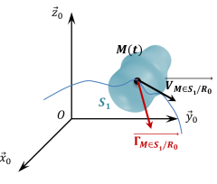
Soit un solide \(S_1\) auquel on associe le repère \(\mathcal{R}_1(O_1,\vec x_1, \vec y_1, \vec z_1)\), en mouvement par rapport au solide \(S_0\) auquel on associe le repère \(\mathcal{R}_0(O_0,\vec x_0, \vec y_0, \vec z_0)\).
Soit un point \(M\) appartenant au solide \(S_1\). L'accélération de ce point \(M\) appartenant au solide \(S_1\) par rapport au solide \(S_0\) est défini par :
\(\boxed{ \quad\overrightarrow{\Gamma_{M\in S_1/\mathcal R_0}}(t) =\left[\dfrac{d\overrightarrow{V_{M\in S_1/S_0}}(t)}{dt}\right]_{\mathcal R_0}\quad }\)
Applications
Mouvement de translation rectiligne
Soit \(M\), un point d'un un solide \(S_1\) en translation rectiligne de direction \(\vec x_0\) par rapport au repère de référence \(\mathcal{R}_0\).
Nous avons vu que dans ce cas :\(\overrightarrow{V_{M\in S_1/\mathcal R_0}}(t) = x'(t) \, \vec x_0\)
Par définition du vecteur accélération , il vient :
\(\overrightarrow{\Gamma_{M\in S_1/S_0}}(t) = \left[\dfrac{d\overrightarrow{V_{M\in S_1/\mathcal R_0}}(t)}{dt}\right]_{\mathcal{R}_0} = \left[\dfrac{d {x'(t) \vec x_0}}{dt}\right]_{\mathcal{R}_0}\)
d'où :\(\boxed{\quad \overrightarrow{\Gamma(M\in S_1/\mathcal R_0)}(t) = x''(t) \, \vec x_0 \quad}\)
Mouvement de rotation autour d'un axe fixe
Soit \(M\), un point d'un un solide \(S_1\) en rotation autour de l'axe fixe\((O,\vec z_0)\) par rapport à au repère de référence \(\mathcal{R}_0\).
Nous avons vu que dans ce cas : \(\overrightarrow{V_{M\in S_1/S_0}}(t) = R \, \theta'(t) \; \vec e_\theta\)
Par définition du vecteur accélération , il vient :
\(\begin{eqnarray*} \, \overrightarrow{\Gamma_{M\in S_1/\mathcal R_0}}(t) & = & \left[\dfrac{d\overrightarrow{V_{M\in S_1/\mathcal R_0}}(t)}{dt}\right]_{\mathcal{R}_0}\\ & = & \left[\dfrac{d {R \, \theta'(t) \; \vec e_\theta}}{dt}\right]_{\mathcal{R}_0}= R \, \left[\dfrac{d { \,\theta'(t) \; \vec e_\theta}}{dt}\right]_{\mathcal{R}_0}\\ &=& R \, \left (\theta''(t) \; \vec e_\theta+\theta'(t) \;\left[\dfrac{d {\vec e_\theta}}{dt}\right]_{\mathcal{R}_0} \right)\end{eqnarray*}\)
Or \(\left[\dfrac{d {\vec e_\theta}}{dt}\right]_{\mathcal{R}_0} = \overrightarrow{\Omega(S_1/S_0)} \wedge \vec e_\theta = \theta'(t)\, \vec z_0 \, \wedge \, \vec e_\theta= - \theta'(t) \, \vec e_r\)
Ainsi,\( \boxed{\quad \overrightarrow{\Gamma_{M\in S_1/S_0}}(t) = R \, \theta''(t) \, \vec e_\theta \, - \, R \, \theta'(t)^2 \, \vec e_r \quad}\)
Remarque : Vocabulaire
Le calcul de \(\overrightarrow{\Gamma_{M\in S_1/\mathcal R_0}}(t)\) met en évidence deux termes :
L'accélération tangentielle : \(\overrightarrow{\Gamma_{T \,(M\in S_1/\mathcal R_0)}}=R \, \theta''(t) \, \vec e_\theta\), tangent à la trajectoire comme son nom l'indique. Il traduit les variations de la norme du vecteur vitesse.
L'accélération normale : \(\overrightarrow{\Gamma_{N \, (M\in S_1/\mathcal R_0)}}=- R \, \theta'(t)^2 \, \vec e_r\) ayant une direction perpendiculaire à celle du vecteur vitesse et orienté vers l’intérieur de la courbure de la trajectoire (vers le centre du cercle ici). Il traduit les variation de direction du vecteur vitesse.
Champ des vecteurs accélération
Soient deux points \(A\) et \(B\) d'un solide \(S_1\) en mouvement par rapport à \(\mathcal R_0\). On rappelle la formule du champ des vecteurs vitesse :
\(\overrightarrow{V_{B\in S_1/\mathcal R_0}} =\overrightarrow{V_{A\in S_1/\mathcal R_0}} +\overrightarrow{BA} \wedge \overrightarrow{\Omega(S_1/S_0)}\)
En dérivant cette expression, par définition du vecteur accélération, on obtient :
\(\overrightarrow{\Gamma_{B\in S_1/\mathcal R_0}} =\overrightarrow{\Gamma_{A\in S_1/\mathcal R_0}} +\left[\dfrac{d\overrightarrow{BA} }{dt}\right]_{\mathcal R_0} \wedge \overrightarrow{\Omega(S_1/S_0)} +\overrightarrow{BA} \wedge \left[\dfrac{d\overrightarrow{\Omega(S_1/S_0)} }{dt}\right]_{\mathcal R_0} \quad (1)\)
\(A\) et \(B\) sont deux point du solide \(S_1\), considéré indéformable donc :
\(\left[\dfrac{d\overrightarrow{BA} }{dt}\right]_{\mathcal R_0}=\underbrace{\left[\dfrac{d\overrightarrow{BA} }{dt}\right]_{\mathcal R_1}}_{= \vec 0}+ \overrightarrow{\Omega(S_1/S_0)} \wedge \overrightarrow{BA}\)
Ainsi (1) devient :
\(\overrightarrow{\Gamma_{B\in S_1/\mathcal R_0}} =\overrightarrow{\Gamma_{A\in S_1/\mathcal R_0}} + \left(\overrightarrow{\Omega(S_1/S_0)} \wedge \overrightarrow{BA} \right)\wedge \overrightarrow{\Omega(S_1/S_0)} +\overrightarrow{BA} \wedge \left[\dfrac{d\overrightarrow{\Omega(S_1/S_0)} }{dt}\right]_{\mathcal R_0}\)
Ou encore : \(\boxed{\overrightarrow{\Gamma_{B\in S_1/\mathcal R_0}} =\overrightarrow{\Gamma_{A\in S_1/\mathcal R_0}} +\overrightarrow{BA} \wedge \left[\dfrac{d\overrightarrow{\Omega(S_1/S_0)} }{dt}\right]_{\mathcal R_0} +\underbrace{\left(\overrightarrow{\Omega(S_1/S_0)} \wedge \overrightarrow{BA} \right)\wedge \overrightarrow{\Omega(S_1/S_0)}}_{\neq \vec 0}}\)
Les vecteurs accélération des points d'un solide ne vérifient pas la relation de changement de point du moment d'un torseur à cause de l'existence du dernier terme \(\left(\overrightarrow{\Omega(S_1/S_0)} \wedge \overrightarrow{BA} \right)\wedge \overrightarrow{\Omega(S_1/S_0)}\). Ainsi, le champ des vecteurs accélération des points d'un solide indéformable n'est pas représentable par un torseur.
Composition des vecteurs accélération
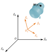
Soit un solide S en mouvement par rapport à deux repères \(\mathcal{R}_0(O_0, \vec x_0, \vec y_0, \vec z_0)\) et \(\mathcal{R}_1(O_1, \vec x_1, \vec y_1, \vec z_1)\), eux même en mouvement l'un par rapport à l'autre.
Soit un point \(M \in S\). Par définition du vecteur accélération :
\(\overrightarrow{\Gamma_{M\in S/\mathcal{R}_0}} =\left[\dfrac{d \overrightarrow{V_{M\in S/\mathcal{R}_0}}}{dt}\right]_{\mathcal{R}_0}\)
Par composition des vecteurs vitesse : \(\quad\overrightarrow{V_{M,S/\mathcal{R}_0}}= \overrightarrow{V_{M,S/\mathcal{R}_1}}+\overrightarrow{V_{M,\mathcal{R}_1/\mathcal{R}_0}}\)
Donc : \(\overrightarrow{\Gamma_{M\in S/\mathcal{R}_0}} = \left[\dfrac{d\overrightarrow{V_{M \in S/\mathcal{R}_1}}}{dt}\right]_{\mathcal{R}_0}+\left[\dfrac{d\overrightarrow{V_{M \in \mathcal{R}_1/\mathcal{R}_0}}}{dt}\right]_{\mathcal{R}_0}\)
Par application du champ des vecteurs vitesse :
\(\overrightarrow{V_{M\in \mathcal{R}_1/\mathcal{R}_0}} =\overrightarrow{V_{O_1\in \mathcal{R}_1/\mathcal{R}_0}} +\overrightarrow{\Omega(\mathcal{R}_1/ \mathcal{R}_0)}\wedge\overrightarrow{O_1M}\)
Donc \(\overrightarrow{\Gamma(M\in S/\mathcal{R}_0)} =\)
\(\underbrace{\left[\dfrac{d\overrightarrow{V_{M \in S/\mathcal{R}_1}}}{dt}\right]_{\mathcal{R}_0}}_{(1)}+ \underbrace{\left[\dfrac{d\overrightarrow{V_{O_1 \in \mathcal{R}_1/\mathcal{R}_0}}}{dt}\right]_{\mathcal{R}_0}}_{(2)}+\underbrace{\left[\dfrac{d \overrightarrow{\Omega(\mathcal{R}_1/ \mathcal{R}_0)}}{dt}\right]_{\mathcal{R}_0} \wedge\overrightarrow{O_1M}}_{(3)}+\underbrace{\overrightarrow{\Omega(\mathcal{R}_1/ \mathcal{R}_0)}\wedge\left[\dfrac{d\overrightarrow{O_1M}}{dt}\right]_{\mathcal{R}_0}}_{(4)}\)
(1) : \(\left[\dfrac{d\overrightarrow{V_{M \in S/\mathcal{R}_1}}}{dt}\right]_{\mathcal{R}_0}=\underbrace{\left[\dfrac{d\overrightarrow{V_{M \in S/\mathcal{R}_1}}}{dt}\right]_{\mathcal{R}_1}}_{= \overrightarrow{\Gamma_{M\in S/\mathcal{R}_1}} }+\overrightarrow{\Omega(\mathcal{R}_1/ \mathcal{R}_0)}\wedge\overrightarrow{V_{M\in S/\mathcal{R}_1}}\)
(2) : \(\left[\dfrac{d\overrightarrow{V_{O_1 \in \mathcal{R}_1/\mathcal{R}_0}}}{dt}\right]_{\mathcal{R}_0} = \overrightarrow{\Gamma_{O_1\in \mathcal{R}_1/\mathcal{R}_0}}\)
(4) : \(\overrightarrow{\Omega(\mathcal{R}_1/ \mathcal{R}_0)}\wedge\left[\dfrac{d\overrightarrow{O_1M}}{dt}\right]_{\mathcal{R}_0}=\overrightarrow{\Omega(\mathcal{R}_1/ \mathcal{R}_0)}\wedge \left( \underbrace{\left[\dfrac{d\overrightarrow{O_1M}}{dt}\right]_{\mathcal{R}_1}}_{= \overrightarrow{V_{M\in S/\mathcal{R}_1}} }+\overrightarrow{\Omega(\mathcal{R}_1/ \mathcal{R}_0)}\wedge\overrightarrow{O_1M} \right)\)
Ainsi
Le terme (IV) peut être simplifié en utilisant l'expression du champ des vecteurs accélération établi au paragraphe 9.3, :
\(\overrightarrow{\Gamma(O_1\in \mathcal{R}_1/\mathcal{R}_0)}+\overrightarrow{\Omega(\mathcal{R}_1/ \mathcal{R}_0)} \wedge \left(\overrightarrow{\Omega(\mathcal{R}_1/ \mathcal{R}_0)} \wedge \overrightarrow{O_1M} \right)+\left[\dfrac{d \overrightarrow{\Omega(\mathcal{R}_1/ \mathcal{R}_0)}}{dt}\right]_{\mathcal{R}_0} \wedge\overrightarrow{O_1M}\)
\(=\overrightarrow{\Gamma(O_1\in \mathcal{R}_1/\mathcal{R}_0)}+\overrightarrow{MO_1} \wedge \left[\dfrac{d \overrightarrow{\Omega(\mathcal{R}_1/ \mathcal{R}_0)}}{dt}\right]_{\mathcal{R}_0} +\left(\overrightarrow{\Omega(\mathcal{R}_1/ \mathcal{R}_0)} \wedge \overrightarrow{MO_1} \right) \wedge \overrightarrow{\Omega(\mathcal{R}_1/ \mathcal{R}_0)}\)
\(=\overrightarrow{\Gamma(M\in \mathcal{R}_1/\mathcal{R}_0)}\)
Au final
Chaque termes de l'équation obtenue porte un nom bien précis :
(I) : accélération absolue
(II) : accélération relative
(III) : accélération de Coriolis
(IV) : accélération d’entraînement.
Remarque :
Cette relation n'est pas à apprendre par cœur. Vous devez en revanche savoir de quoi est composée une accélération, identifier et nommer les différents termes du résultat. Vous devez donc savoir refaire ce calcul.