Composition des mouvements
Composition des vecteurs vitesse
Fondamental : Composition des vecteurs vitesse
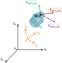
Soit un solide \(S_2\) auquel on associe le repère \(\mathcal{R}_2(O_2,\vec x_2, \vec y_2, \vec z_2)\) en mouvement par rapport à deux solides \(S_0\) et \(S_1\) auxquels on associe respectivement les repères \(\mathcal{R}_0(O_0,\vec x_0, \vec y_0, \vec z_0)\) et \(\mathcal{R}_1(O_1,\vec x_1, \vec y_1, \vec z_1)\)
Pour tout point M appartenant au solide \(S_2\), on a :
\(\boxed{\quad\overrightarrow{V_{M,S_2/\mathcal{R}_0}}= \overrightarrow{V_{M,S_2/\mathcal{R}_1}}+\overrightarrow{V_{M,\mathcal{R}_1/\mathcal{R}_0}} \quad }\)
Remarque : Vocabulaire
\(\overrightarrow{V_{M,S_2/\mathcal{R}_0}}\) est appelé vecteur vitesse absolue ;
\(\overrightarrow{V_{M,S_2/\mathcal{R}_1}}\) est appelé vecteur vitesse relative ;
\(\overrightarrow{V_{M,\mathcal{R}_1/\mathcal{R}_0}}\) est appelé vecteur vitesse d'entraînement. Il correspond à la vitesse du point \(M\) imaginé fixe dans \(\mathcal R_1\) dans le mouvement de \(S_1\) par rapport à \(\mathcal R_0\).
Complément : Démonstration
\(\begin{eqnarray*}\quad\overrightarrow{V_{M,S_2/S_0}} & = &\left[\dfrac{d\overrightarrow{O_0 M}}{dt}\right]_{\mathcal{R}_0}=\underbrace{\left[\dfrac{d\overrightarrow{O_0O_1(t)}}{dt}\right]_{\mathcal{R}_0}}_{\overrightarrow{V_{O_1\in S_1/\mathcal{R}_0}} }+\underbrace{\left[\dfrac{d\overrightarrow{O_1M(t)}}{dt}\right]_{\mathcal{R}_0}}_{\rightarrow \text{ dérivation vectorielle}} \\& = & \overrightarrow{V_{O_1\in S_1/\mathcal{R}_0}} +\underbrace{\left[\dfrac{d\overrightarrow{O_1M(t)}}{dt}\right]_{\mathcal{R}_1}}_{\overrightarrow{V_{M\in S_2/\mathcal{R}_1}}}+ \overrightarrow{\Omega(S_1/S_0)}\wedge \overrightarrow{O_1M(t)}\\\end{eqnarray*}\)
Or d'après le champ des vecteurs vitesses :
\(\begin{eqnarray*}\overrightarrow{V_{M\in \mathcal R_1/\mathcal R_0}} & = &\overrightarrow{V_{O_1\in \mathcal R_1/\mathcal R_0}} +\overrightarrow{M(t)O_1} \wedge\overrightarrow{\Omega(S_1/S_0)} \\& = & \overrightarrow{V_{O_1\in \mathcal R_1/\mathcal R_0}} +\overrightarrow{\Omega(S_1/S_0)}\wedge \overrightarrow{O_1M(t)}\\\end{eqnarray*}\)
Ainsi : \(\begin{eqnarray*}\boxed{\quad\overrightarrow{V_{M,S_2/\mathcal R_0}}= \overrightarrow{V_{M,S_2/\mathcal R_1}}+\overrightarrow{V_{M,\mathcal R_1/\mathcal R_0}} \quad }\end{eqnarray*}\)

Fondamental : Généralisation
La composition du vecteur vitesse peut se généraliser avec n solides :

Composition des vecteurs taux de rotation
Fondamental : Composition des vecteurs taux de rotation
Soient deux solides \(S_1\) et \(S_2\) en mouvement par rapport à un solide \(S_0\) . On a :
Complément : Démonstration
Soit un vecteur \(\vec u\) quelconque (non nul). Soient trois solides \(S_2, S_1\) et \(S_0\) en mouvements relatifs. \(\overrightarrow{\Omega(S_2/S_0)}, \overrightarrow{\Omega(S_1/S_0)} \, \text{ et } \, \overrightarrow{\Omega(S_2/S_1)}\) sont supposés non nuls.
D'après la formule de la base mobile entre les base 1 et 0 et entre les bases 2 et 1 :
\(\left[\dfrac{d\vec u}{dt}\right]_{S_0} = \left[\dfrac{d\vec u}{dt}\right]_{S_1}+ \overrightarrow{\Omega(S_1/S_0)}\wedge {\vec u}\quad (1)\quad\) et \(\left[\dfrac{d\vec u}{dt}\right]_{S_1} = \left[\dfrac{d\vec u}{dt}\right]_{S_2}+ \overrightarrow{\Omega(S_2/S_1)}\wedge {\vec u} \quad (2)\)
Ainsi, en injectant (2) dans (1) \(\left[\dfrac{d\vec u}{dt}\right]_{S_0} = \left[\dfrac{d\vec u}{dt}\right]_{S_2}+\left( \overrightarrow{\Omega(S_2/S_1)}+\overrightarrow{\Omega(S_1/S_0)} \right) \wedge {\vec u} \quad \quad (3)\)
De plus, toujours d'après la formule de la base mobile mais cette fois entre les base 2 et 0 :
\(\left[\dfrac{d\vec u}{dt}\right]_{S_0} = \left[\dfrac{d\vec u}{dt}\right]_{S_2}+ \overrightarrow{\Omega(S_2/S_0)}\wedge {\vec u} \quad \quad (4)\)
\(\begin{eqnarray*} \text{Ainsi, } \quad (3) = (4) &\Leftrightarrow & \left[\dfrac{d\vec u}{dt}\right]_{S_2}+ \overrightarrow{\Omega(S_2/S_0)}\wedge {\vec u} = \left[\dfrac{d\vec u}{dt}\right]_{S_2}+( \overrightarrow{\Omega(S_2/S_1)}+\overrightarrow{\Omega(S_1/S_0)})\wedge {\vec u} \\ & \Leftrightarrow & \left(\overrightarrow{\Omega(S_2/S_0)}-\left( \overrightarrow{\Omega(S_2/S_1)}+\overrightarrow{\Omega(S_1/S_0)} \right) \right) \wedge \vec u=\vec 0 \\ &\Leftrightarrow & \overrightarrow{\Omega(S_2/S_0)}-\left( \overrightarrow{\Omega(S_2/S_1)}+\overrightarrow{\Omega(S_1/S_0)} \right)=\vec 0 \, \text{, car}\, \vec u \text{ est quelconque}\\ &\Leftrightarrow & \boxed{\overrightarrow{\Omega(S_2/S_0)}= \overrightarrow{\Omega(S_2/S_1)}+\overrightarrow{\Omega(S_1/S_0)}} \end{eqnarray*}\)
Fondamental : Généralisation
La composition du vecteur taux de rotation peut se généraliser avec n solides :
Cas du mouvement hélicoïdal
Un mouvement hélicoïdal est la combinaison d'une rotation autour d'un axe fixe et d'un translation rectiligne de même axe. :
Soit \(\mathcal{R}_1\) un repère associé à un solide en mouvement de translation rectiligne de direction \(\vec z_0\) par rapport au repère de référence \(\mathcal{R}_0\) :
\(\overrightarrow{\Omega(\mathcal R_1/\mathcal R_0)}=\vec 0\quad (1a)\)
\(\overrightarrow{V_{M,\, \mathcal R_1/\mathcal R_0}}= z'(t) \, \vec z_0 \quad (1b)\)
Soit \(S_2\) un solide auquel on associe le repère \(\mathcal{R}_2\), en mouvement de rotation d'axe \((O,\vec z_1)\) par rapport au repère \(\mathcal{R}_1\) :
\(\overrightarrow{\Omega(S_2/\mathcal R_1)}=\omega_{2/1} \, \vec z_1\), avec \(\omega_{2/1} =\theta'_{2/1}(t)\quad (2a)\)
\(\overrightarrow{V_{M,\mathcal S_2/\mathcal R_1}}\, = R \, \omega_{2/1}\, \vec y_2 \quad (2b)\)
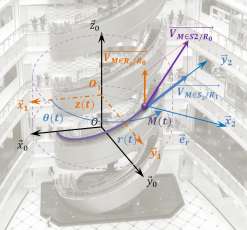
Ainsi en composant les mouvement de \(S_2/\mathcal R_1\) et de \(\mathcal R_1/\mathcal R_0\) on peut déterminer le vecteur taux de rotation et le vecteur vitesse d'un point \(M\)dans le mouvement hélicoïdal d'axe \((O_0, \vec z_0)=(O_1,\vec z_1)\)de \(S_2\) par rapport au repère de référence \(\mathcal R_0\) :
\(\overrightarrow{\Omega(S_2/\mathcal R_0)} = \overrightarrow{\Omega(S_2/\mathcal R_1)}+\overrightarrow{\Omega(\mathcal R_1/\mathcal R_0)} = \omega_{2/1} \, \vec z_1 + \vec 0 \quad\)
et donc : \(\boxed{\overrightarrow{\Omega(S_2/\mathcal R_0)} =\omega_{2/1} \, \vec z_1}\)
\(\overrightarrow{V_{M,\mathcal S_2/\mathcal R_0}}\, = \overrightarrow{V_{M,S_2/\mathcal R_1}}+\overrightarrow{V_{M,\mathcal R_1/\mathcal R_0}}\)
Soit : \(\boxed{\overrightarrow{V_{M,\mathcal S_2/\mathcal R_0}}\, =R \, \omega_{2/1}\, \vec y_2 \quad + z'(t) \, \vec z_0}\)
La trajectoire d'un point quelconque du solide S en mouvement hélicoïdal autour d'un axe fixe par rapport à un repère R est une hélice circulaire dont l'axe correspond à celui de la rotation et de la translation.